Today we shall look at the first sampling method we introduced: Simple Random Sampling. Recall that we mentioned that this is the most basic form of probability sampling since it provides the theoretical basis for the more complicated forms. Here we will look at how to select a simple random sample (SRS) and also estimate the population parameters for SRS too.
Before that, we will look at the notations that we will be using:
- N: the total number of elements in the population (or Universe, depending on what you’re looking at)
- U = {1, 2, …, N}: the index set for the elements in the population. Recall the assumptions we made previously, this implies that U is just the sampling frame.
- n: sample size. N = n iff its the census.
- D: sample index set
Put the above together, we say a simple random sample with size n is sample index set D from U.
Next, I will introduce two types of SRS:
- SRS with replacement: Return the unit after drawing, repeat n time.
- SRS without replacement: Draw n distinct units for a sample size of n.
Clearly, we are interested to do SRS without replacement, so I will only discuss this.
Since every unit is equally likely to be selected, we consider the following definition
- Unit Inclusion Probability,


- The probability of selecting a sample index D of n units is
 . We note that we have
  possible samples here.
Now our next task is to learn how to use the sample to estimate the population parameters, i.e, population mean, proportion, total, variance, standard deviation, coefficient of variation.
- Estimating Population Mean,

Estimator,
You should notice that this is the same as the sample mean,
Loosely speaking, the mean of a mean, is the mean itself. 🙂 - Estimating Population proportion, p
Estimator,
- Estimating Population total, t
Estimator,
Here, , which measures how many units are represented by the sampled unit since
  is the inclusion probability.
 - Estimating Population variance,

Estimator,
After finding these estimators, we need to assess the quality of our estimates. We want our estimators to have the following properties:
- Low or no bias and high precision
- Low bias or no biased (unbiased): Expectation (mean) of all estimates across samples is close or equal to the population parameter
- High precision (low variance): Variations in estimates across samples is small
So you might notice I used the phrase “estimates across samples”. Recall that we assume a finite population, so we can write down all possible samples of size n with respective probability. Here, our estimator can be described by a discrete probability distribution, which gives us a sampling distribution for our estimator. The sampling distribution is used to assess the quality (mentioned above) of the estimator. Now we look at how to determine them quantitatively. Note here that  refers to the population parameter for convenience.
- Bias: The expectation of the estimator
 is the mean of the sampling distribution of
  .
.
Estimation bias:
If , the estimator is unbiased.
 - Variance

Clearly, we hope that the value here is small. - Mean Squared Error (MSE)

Notice that MSE is a takes into account both the variance and the bias for calculation.
Qualities of Estimator
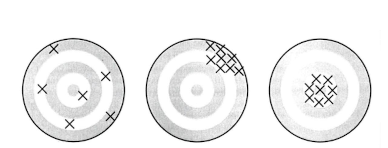
Qualitatively, unbiased (no bias) means that the average position of all arrows is at the bull’s eye. But may have big variance. Precise (small variance) means all arrows are close together, but may be away from the bull’s eye. Accurate (small MSE) mean all arrows are close together (small variance) and near the centre of the target (small bias). We thus have the following conclusions:
An estimator of is unbiased if  , precise if is small, and accurate if
  is small.
Note that a badly biased estimator may be precise, but it will not be accurate, as accuracy (MSE) is how close the estimate is to the true value, while precision (variance) is how close estimates from different samples are to each other.
We will look at how to investigate these qualities next.
Sampling & Survey #1 – Introduction
Sampling & Survey #2 – Simple Probability Samples
Sampling & Survey #3 – Simple Random Sampling
Sampling & Survey #4 – Qualities of estimator in SRS
Sampling & Survey #5 – Sampling weight, Confidence Interval and sample size in SRS
Sampling & Survey #6 – Systematic Sampling
Sampling & Survey #7 – Stratified Sampling
Sampling & Survey # 8 – Ratio Estimation
Sampling & Survey # 9 – Regression Estimation
Sampling & Survey #10 – Cluster Sampling
Sampling & Survey #11 – Two – Stage Cluster Sampling
Sampling & Survey #12 – Sampling with unequal probabilities (Part 1)
Sampling & Survey #13 – Sampling with unequal probabilities (Part 2)
Sampling & Survey #14 – Nonresponse