SRS form the basis of sampling and survey methods as it is easy to design and analyse, but it is rarely the best design. We may adopt systematic sampling or cluster sampling but we often are limited by the availability of sampling from. Thus, we need to look at stratified sampling to increase the precision.
In stratified sampling, we divide the population in H subpopulations, called strata, which do not overlap (mutually exclusive) and constitute the whole population so that each sampling unit belongs to exactly one stratum. We then draw independent random sample from each stratum.
Consider that we have 1000 males and 1000 females to select from, a SRS of size 100 might lead us to have no or very few males or females. This will cause us to not have a presentative sample since men and women respond differently on the item of interest. A stratified sample on the other hand, will suggest we take a SRS of 50 males and an independent SRS of 50 females, ensuring that the proportion in the sample is the same as that in the population.
- Clearly, we will have better precision (lower variance) using a stratified sampling as compared to SRS, for the estimates of population means and total. This is because variance within each stratum is often lower than ht variance in the whole population.
- Convenient to administer and may result in a lower cost. Sampling frame may be conducted differently in different strata, or different sampling designs or field procedures may be used. For example, using an internet survey by a large firm and a telephone survey for a small firm.
So let us look at some notations that we will be using. Firstly, we divide the population N into H mutually exclusive and exhaustive strata.
h = 1, 2, …, H index the strata.
 = number of sampling units in stratum h. Total number of units in the entire population
 = number of sample units draw from stratum h. Total sample size
 = the set of
  sample units drawn from stratum h.
 = value of
  unit in stratum h, where h = 1, 2, .., H and j = 1, 2, …, .
Stratum population total, 
Population total, 
Stratum population mean, 
Population mean, 
Stratum population variance, 
Since we assume SRS within each stratum, then when we have a population of units and take an SRS of units, we can estimate  by
by  and
and  by
by 
Estimate of stratum population mean , 
Estimate of stratum population total , 
Estimate of stratum population variance  ,
, 
Notice  appears a few times, this is the weight of which is the proportion of the population units in stratum h, that is, relative sizes of the strata. When we use stratified sampling, the relative sizes of the strata must be known.
Estimate of population total , 
Estimate of population mean  ,
, 
Since we do SRS in each stratum, both  and
and  are unbiased estimates of and t. Similarly, the variances of the estimators are obtained through SRS since we do independent sampling for different strata.


As always, the standard error of an estimator is the square root of the estimated variance:


As long as we select at least one element per stratum, the specification for a stratified sample is satisfied. And with two elements per stratum, we can estimate both the mean and its error.
If either the sample sizes within each stratum are large or the number of strata are large, the approximate  confidence interval for the population mean can be constructed as
  =
= 
We recall that proportion is a special mean.


In SRS, we learnt that  and
and  for i = 1, 2, …, N, refers to our sample weights. The sampling weight of unit i can be interpreted as the number of population units represented by unit i. And in STR:

Here  measures the number of units in population represented by the unit in stratum h. Clearly,
It should be noted that under SRS within strata, weights for each sampling unit within a stratum are the same, while weights across the strata may be different.
Now we study how to do proportional allocation (an important property of stratified sampling), that is, allocating such that the number of sampled units in each stratum is proportional to the size of the stratum.
Stratum sample size, 
Notice this rewrites to  which implies that sampling weights (inclusion probabilities) for all units are constant.
Thus, the probability that an individual will be selected to be in the sample,  is the same as in an SRS, but many bad samples that could occur in an SRS cannot be elected in a stratified sample with proportional allocation. A stratified sampled with proportional allocation is self-weighting (every unit in the sample has the same weight and represents the same number of unit in the population).
When is large enough, the variance of is under proportional allocation is usually lesser or equal to the variance of  from an SRS with the same number of observations.
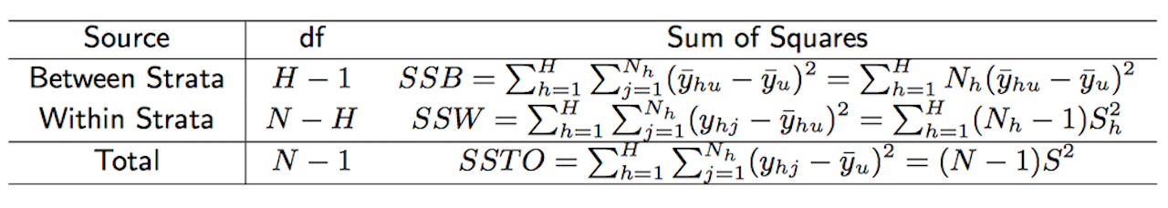
Sum of Squares
When we have a stratified sample of size n with proportional allocation,

We can find  too.
too.
In general, the variance of the estimator of t from a stratified sample with proportional allocation will be smaller than the variance of the estimator of t from an SRS with the same number of observations. The more unequal the stratum means the more precise get when we use proportional allocation.
Note that  depends primarily on SSW since SSTO is a fixed value for the finite population. Consequently, SSW is smaller when SSB is larger. This result ONLY holds for population variances.
After considering proportional allocation, we can now look at optimal allocation. For proportional allocation, we increase precision (lower variance) when the within-stratum variance are more of less equal across all the strata. But we do not consider the cost  here. Our goal is to minimise the variance of the estimate given a total cost.
Problem: min  where C = total cost,
  = overhead (fixed) cost and = cost of taking an observation in stratum h.
We can use Lagrange Multpliers to solve and will find that the optimal allocation 
Thus the optimal sample size in stratum h is 
Since , we see that sample size depends on stratum size, stratum variance, sampling cost.
- Proportional allocation is the optimal allocation if all variance and cost are equal across the strata.

- Neyman allocation is a special case of optimal allocation, used when the cost in the strata (not the variances) are approximately equal.

In short, we have 3 methods of allocation of a sample to strata: Equal, Proportional, and Optimum (Neyman). These allocation strategies allow us to know the proportion of sample allocated to every stratum.
We say under absolute precision, that the desired margin of error is half-width of the confidence interval. The half-width of CI is  by definition if we ignore the FPC. So
We may argue that stratified sampling almost always gives higher precision than SRS, and one should simply consider stratified only. However, we should note that stratified adds complexity to the survey, and we need to weigh if the gain in precision is worthy as compared with the added complexity. Stratified sampling is most efficient when the stratum mean differ widely, so we should construct such that the strata mean is as different as possible. To do this, we need more information. But the more information we have, the more strata we have, the more complexity there is. We will use SRS if there is no or little information about the target population.
Sampling & Survey #1 – Introduction
Sampling & Survey #2 – Simple Probability Samples
Sampling & Survey #3 – Simple Random Sampling
Sampling & Survey #4 – Qualities of estimator in SRS
Sampling & Survey #5 – Sampling weight, Confidence Interval and sample size in SRS
Sampling & Survey #6 – Systematic Sampling
Sampling & Survey #7 – Stratified Sampling
Sampling & Survey # 8 – Ratio Estimation
Sampling & Survey # 9 – Regression Estimation
Sampling & Survey #10 – Cluster Sampling
Sampling & Survey #11 – Two – Stage Cluster Sampling
Sampling & Survey #12 – Sampling with unequal probabilities (Part 1)
Sampling & Survey #13 – Sampling with unequal probabilities (Part 2)
Sampling & Survey #14 – Nonresponse
[…] Confidence Interval and sample size in SRS Sampling & Survey #6 – Systematic Sampling Sampling & Survey #7 – Stratified Sampling Sampling & Survey # 8 – Ratio Estimation Sampling & Survey # 9 – Regression […]