Continuous Random Variables

We look at the definitions first.

A continuous random variable, X, has a probability density function (PDF), $f(\bullet)$ if $f(x) \ge 0$ and for all events A
$P(X \in A) = \int_A f(y) dy$
The CDF and PDF are related by $F(x) = \int_{-\infty}^x f(y) dy$
It is good to know that we have $P(X \in (x - \frac{\epsilon}{2}, x + \frac{\epsilon}{2})) \approx \epsilon f(x)$

We X has a normal distribution, $X \sim N(\mu, {\sigma}^2)$ , and $f(x) = \frac{1}{\sqrt{2 \pi {\sigma}^2}}e^(-\frac{(x - \mu)^2}{2 {\sigma}^2})$ . And $\mathbb{E}[X] = \mu$ while $Var(X) = {\sigma}^2$

Log normal Distribution Source: www.me.utexas.edu

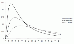
We also have the log-normal distribution, $X \sim LN (\mu, {\sigma}^2)$ and $log(X) \sim N(\mu, {\sigma}^2)$ . Here, $\mathbb{E} [X] = e^(\mu + \frac{{\sigma}^2}{2})$ and $Var(X) = e^(2 \mu + {\sigma}^2) (e^{{\sigma}^2} - 1)$ . The log-normal distribution is very important in financial applications, for starters, the Black Scholes Equation.

About

KS Teng

KS has been teaching H2/H1 Mathematics and IB mathematics for almost two decades. Having taught students from all various Junior Colleges, KS adapts to students' abilities and help them better understand the topics. As someone who loves to teach mathematics and sees it as a truly useful tool in life, KS seeks to enable students to appreciate math. Therefore, his tuition mission is to motivate and cultivate students to be independent and confident thinkers.

Comments

pingbacks / trackbacks

Conditional Expectations and Variances – The Culture
[…] we look at an important concept that is an extension from Bayes Theorem, which we discussed […]
January 19th, 2016 04:00 PM

Cart

Continuous Random Variables

Leave a Comment
Cancel reply

Continuous Random Variables

Leave a Comment Cancel reply

Leave a Comment
Cancel reply