As usual, definitions first.
The cumulative distribution function (CDF), ![]() of a random variable, X, is defined by
of a random variable, X, is defined by
![]()
A discrete random variable, X, has probability mass function (PMF), ![]() , if
, if ![]() and for all events A we have
and for all events A we have ![]()
The expected value of a discrete random variable, X is given by
![]()
The variance of an random variable, X, is defined as ![]()
- Binomial Distribution
We say the X has a binomial distribution, that is, ![]() , if
, if ![]()
For example, X can represent the number of heads in n independent coin tosses, where ![]() . We have that the mean
. We have that the mean ![]() and variance
and variance ![]()
A simpler case of binomial where there is only one event is called the Bernoulli distribution.
I’ll give a simple illustration of binomial model used in finance. This was also used in finance engineering in the beginning.
Suppose a fund manager outperforms the market in a given year with probability p and under performs the market with probability 1 – p. She has a track record of 10 years and has outperformed the market in 8 out of 10 years. We also note that performance in any one year is independent of performance in other years.
From this illustration, we note that there are only two outcomes, she outperforms or underperforms. We can let X be the number of outperforming years. Assuming the fund manager has no skill, ![]() and we can find
and we can find ![]() to find out the probability that she outperforms at least 8 out of 10 years.
to find out the probability that she outperforms at least 8 out of 10 years.
An extension here will be to consider there are M fund managers instead of 1 now.
- Poisson Distribution
-
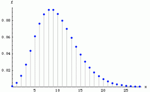
We say that X has a
Next, we look at Bayes Theorem, also known as “conditional probability” in H2 Mathematics.
Let A and B be two events for which ![]() . Then
. Then
![]()
![]()
![]()
where ![]() ‘s form a partition of the sample space.
‘s form a partition of the sample space.


[…] Discrete Random Variables […]